Connecting other packages
We can utilise the data generate in Cecelia with other packages for further detailed downstream analysis. Many of these will be specialised R/python packages. The idea behind this is that the user can define and verify all their populations within the GUI while an analyst might want to delve deeper into the structure and components of these populations.
We have tried to create functions that the conversion between Cecelia populations and other packages is relatively straightforward. These detailed analysis steps could then be integrated within the Cecelia GUI to make them available to people without scripting/programming knowledge. In this sense we envision that the package will grow to fit the needs of their users.
R packages
SPIAT
SPIAT is an R-package that simplifies commonly used spatial analysis methods for multiplex imaging. Here, we use the example Mouse spleen confocal after LCMV infection to look at populations from conventional confocal images.
 1library(cecelia)
 2cciaUse("~/cecelia")
 3
 4# init ccia object
 5cciaObj <- initCciaObject(
 6  pID = pID, uID = "6QzZsl", versionID = versionID, initReactivity = FALSE
 7)
 8
 9uIDs <- names(cciaObj$cciaObjects())
10
11# get pops
12pops <- cciaObj$popPaths(popType = "flow", includeFiltered = FALSE, uIDs = uIDs[1])
13
14# exclude 'O' pops
15pops <- pops[is.na(str_match(pops, "/O[0-9]*$"))]
16pops <- pops[is.na(str_match(pops, "/nonDebris$"))]
17
18spe <- cciaObj$spe(popType = "flow", pops = pops, uIDs = uIDs)
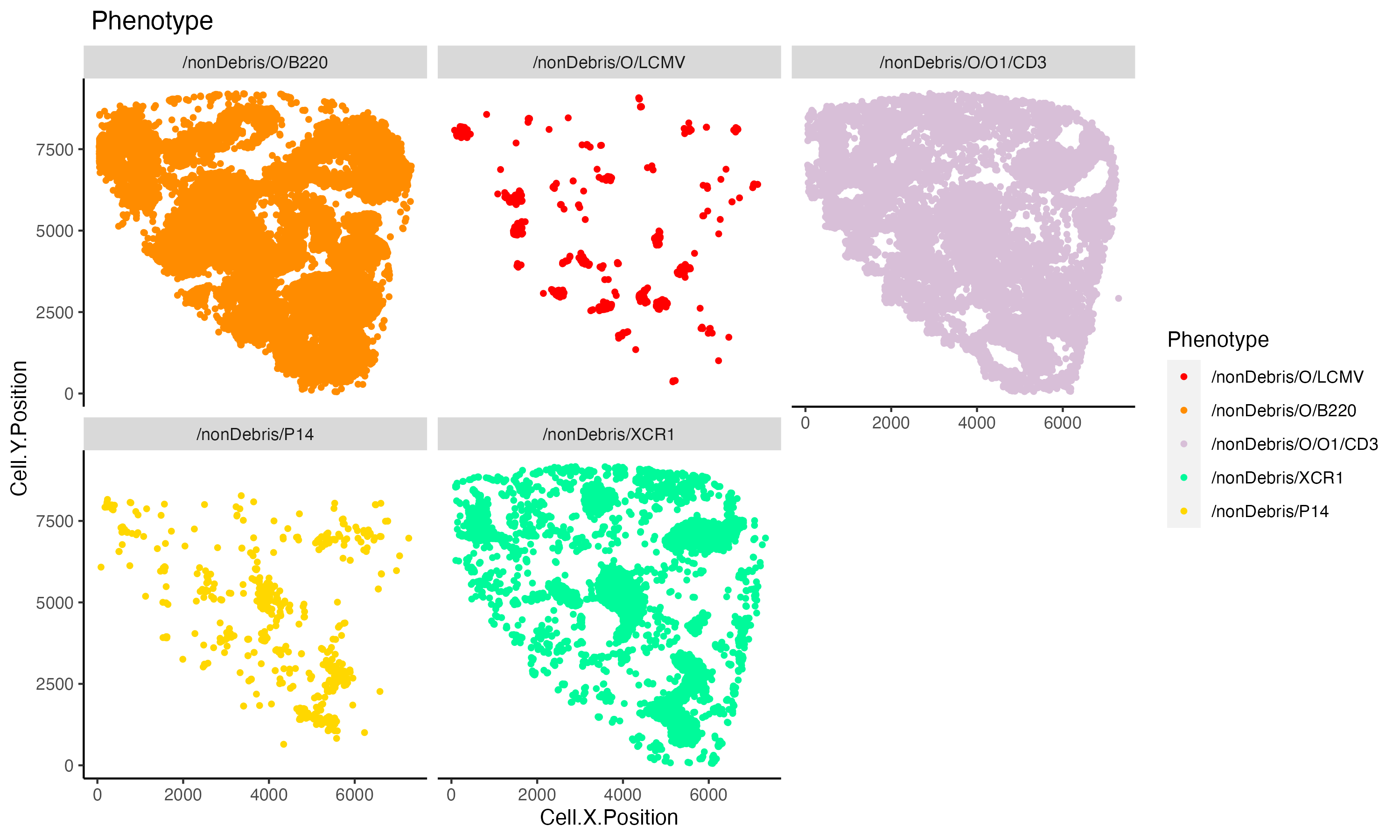
 1# get reference object to show image from set
 2x <- cciaObj$cciaObjects(uIDs = c("NjumBK"))[[1]]
 3imPopMap <- x$imPopMap(popType = "flow", includeFiltered = TRUE)
 4popColours <- sapply(imPopMap, function(x) {x$colour})
 5names(popColours) <- sapply(imPopMap, function(x) {x$path})
 6
 7phenotypes <- unique(spe[[1]]$Phenotype)
 8popColours <- popColours[names(popColours) %in% phenotypes]
 9
10# plot populations
11SPIAT::plot_cell_categories(spe$NjumBK, pops, popColours, "Phenotype") +
12  facet_wrap(.~Phenotype)
 1# get entropies
 2gradient_pos <- seq(20, 300, 20) # radii
 3
 4spiat.entropies <- lapply(spe[names(spe) == "NjumBK"], function(x) {
 5  as.data.table(SPIAT::entropy_gradient_aggregated(
 6    x, cell_types_of_interest = pops,
 7    feature_colname = "Phenotype", radii = gradient_pos)$gradient_df)
 8})
 9
10entropiesDT <- rbindlist(spiat.entropies, idcol = "uID")
 1datToPlot <- entropiesDT %>%
 2  pivot_longer(
 3    cols = starts_with("Pos_"),
 4    names_to = "radius",
 5    names_pattern = ".*_(.*)",
 6    values_to = "value") %>%
 7  mutate(radius = as.numeric(radius))
 8
 9ggplot(datToPlot, aes(radius, value, color = Celltype2, fill = Celltype2, group = Celltype2)) +
10  theme_classic() +
11  geom_line(size = 1.5) +
12  # geom_smooth() +
13  facet_grid(uID~Celltype1) +
14  scale_color_brewer(palette = "Set1") +
15  scale_fill_brewer(palette = "Set1")
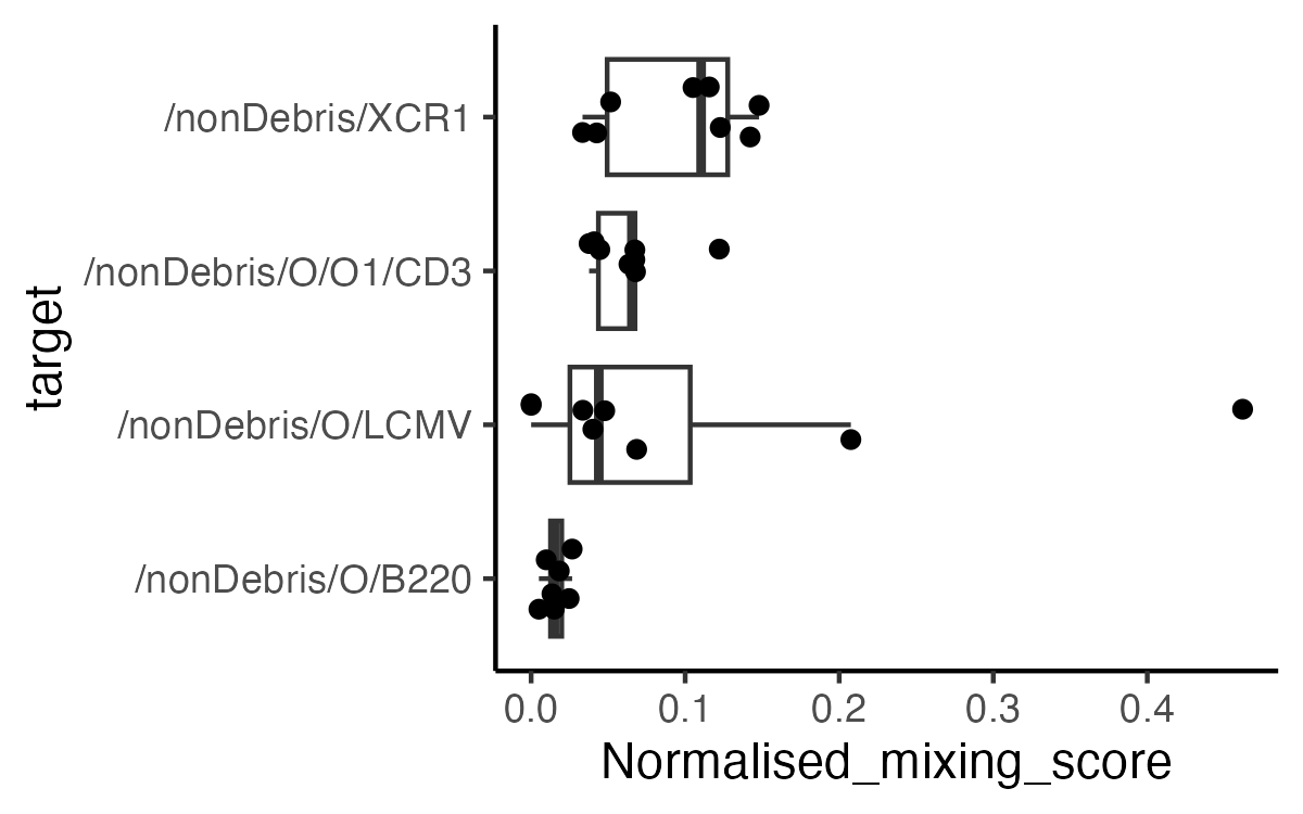
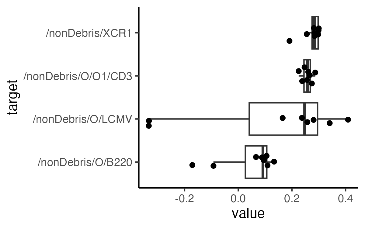
 1# Normalized mixing score (NMS)
 2target_pops <- pops[pops != "/nonDebris/P14"]
 3spiat.nms <- lapply(target_pops, function(x) {
 4  nsm <- lapply(spe, function(y) {
 5    as.data.table(SPIAT::mixing_score_summary(
 6      spe_object = y,
 7      reference_celltype = "/nonDebris/P14",
 8      target_celltype = x,
 9      feature_colname = "Phenotype"))
10  })
11
12  rbindlist(nsm, idcol = "uID")
13})
14names(spiat.nms) <- target_pops
15spiat.nmsDT <- rbindlist(spiat.nms, idcol = "target")
16
17ggplot(spiat.nmsDT, aes(target, Normalised_mixing_score)) +
18  theme_classic() +
19  geom_boxplot(outlier.alpha = 0) +
20  geom_jitter(
21    # position = position_jitterdodge(jitter.width = 0.10), alpha = 1.0) +
22    width = 0.2, alpha = 1.0) +
23  coord_flip()
 1# Cross-K AUC
 2spiat.auc <- lapply(target_pops, function(x) {
 3  auc <- lapply(spe, function(y) {
 4    SPIAT::AUC_of_cross_function(SPIAT::calculate_cross_functions(
 5      spe_object = y,
 6      method = "Kcross", cell_types_of_interest = c("/nonDebris/P14", x),
 7      dist = 100,
 8      feature_colname = "Phenotype"))
 9  })
10
11  DT <- as.data.table(as.data.frame(unlist(auc)) %>% rownames_to_column())
12  colnames(DT) <- c("uID", "value")
13  DT
14})
15names(spiat.auc) <- target_pops
16spiat.aucDT <- rbindlist(spiat.auc, idcol = "target")
17
18ggplot(spiat.aucDT, aes(target, value)) +
19  theme_classic() +
20  geom_boxplot(outlier.alpha = 0) +
21  geom_jitter(
22    # position = position_jitterdodge(jitter.width = 0.10), alpha = 1.0) +
23    width = 0.2, alpha = 1.0) +
24  coord_flip()
spatstat
spatstat is a collection of R-packages that enable complex analysis of spatial patterns. To illustrate how to work with this package we are using the same dataset as for SPIAT above.
 1library(cecelia)
 2cciaUse("~/cecelia")
 3
 4# init ccia object
 5cciaObj <- initCciaObject(
 6  pID = pID, uID = "6QzZsl", versionID = versionID, initReactivity = FALSE
 7)
 8
 9exp.info <- as.data.table(cciaObj$summary(withSelf = FALSE, fields = c("Attr")))
10uIDs <- exp.info$uID
11
12# get pops
13pops <- cciaObj$popPaths(popType = "flow", includeFiltered = FALSE, uIDs = uIDs[1])
14
15# # exclude 'O' pops
16pops <- pops[is.na(str_match(pops, "/O[0-9]*$"))]
17pops <- pops[is.na(str_match(pops, "/nonDebris$"))]
18windowPops <- c("root")
19
20# get ppp for all populations
21popPPP <- lapply(pops, function(x) {
22  cciaObj$ppp(
23    popType = "flow", pops = x, uIDs = uIDs, usePhysicalScale = FALSE, windowPops = windowPops)
24})
25names(popPPP) <- pops
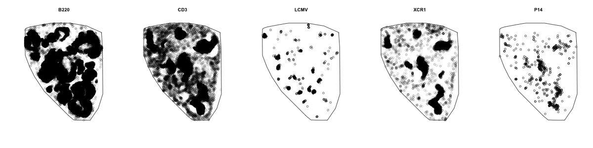
1# plot populations out
2layout(matrix(1:5, ncol = 5))
3plot(popPPP$`/nonDebris/O/B220`$NjumBK, main = "B220")
4plot(popPPP$`/nonDebris/O/O1/CD3`$NjumBK, main = "CD3")
5plot(popPPP$`/nonDebris/O/LCMV`$NjumBK, main = "LCMV")
6plot(popPPP$`/nonDebris/XCR1`$NjumBK, main = "XCR1")
7plot(popPPP$`/nonDebris/P14`$NjumBK, main = "P14")
1# test for spatial randomness
2ce.results <- list()
3for (i in names(popPPP)) {
4  message(paste(">> Test CSR for", i))
5  # test for randomness
6  ce.results[[i]] <- unlist(parallel::mclapply(popPPP[[i]], function(x) {
7    spatstat.explore::clarkevans.test(x, method = "MonteCarlo", nsim = 99)$statistic
8  }))
9}
 1# plot out
 2cdDF <- as.data.frame(ce.results)
 3colnames(cdDF) <- stringr::str_extract(colnames(cdDF), "(?<=\\.)[^\\.]*$")
 4rownames(cdDF) <- stringr::str_extract(rownames(cdDF), ".+(?=\\.R)")
 5
 6ggplot(cdDF %>% pivot_longer(cols = everything(), names_to = "pop", values_to = "ce"),
 7       aes(pop, ce)) +
 8  theme_classic() +
 9  geom_boxplot(outlier.alpha = 0) +
10  geom_jitter(width = 0.2, alpha = 1.0) +
11  expand_limits(y = 0) + geom_hline(yintercept = 1)

celltrackR
celltrackR is an R-package to facilitate analysis of cell tracks. Here we are using the Mouse lymph node HSV infection dataset to illustrate its basic usage in the context of Cecelia.
 1library(cecelia)
 2cciaUse("~/cecelia")
 3
 4# init ccia object
 5cciaObj <- initCciaObject(
 6  pID = pID, uID = "rXctjl", versionID = versionID, initReactivity = FALSE
 7)
 8
 9# get experimental info
10exp.info <- as.data.table(cciaObj$summary(
11  withSelf = FALSE, fields = c("Attr")
12))
13
14uIDs <- exp.info[Cells == "gDT_gBT" & Include == "Y"]$uID
15
16# get tracks for analysis
17tracks.list <- lapply(
18  list(gBT = "gBT", gDT = "gDT"), function(x) cciaObj$tracks(pop = x, uIDs = uIDs))
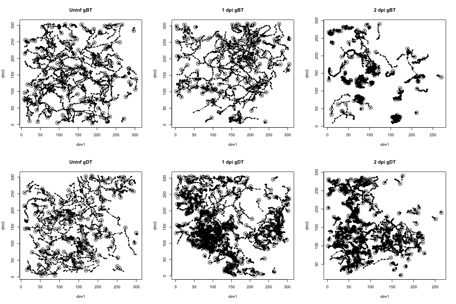
1# plot out tracks
2layout(matrix(1:6, ncol = 3))
3plot(tracks.list$gBT$fizPPH, col = 1, main = "Uninf gBT") # Uninf
4plot(tracks.list$gDT$fizPPH, col = 1, main = "Uninf gDT") # Uninf
5plot(tracks.list$gBT$`2nFwDR`, col = 1, main = "1 dpi gBT") # dpi 1
6plot(tracks.list$gDT$`2nFwDR`, col = 1, main = "1 dpi gDT") # dpi 1
7plot(tracks.list$gBT$LfVNe6, col = 1, main = "2 dpi gBT") # dpi 2
8plot(tracks.list$gDT$LfVNe6, col = 1, main = "2 dpi gDT") # dpi 2
 1# get normalised tracks to plot
 2tracks.DT.norm <- tracks.combine.dt(lapply(
 3  tracks.list, function(x) tracks.apply.fun(x, celltrackR::normalizeTracks)
 4))
 5
 6ggplot(tracks.DT.norm %>% left_join(exp.info),
 7       aes(x, y, group = interaction(uID, track_id))) +
 8  # geom_point(size = 0.5) +
 9  geom_path(size = 0.1, colour = "black") +
10  theme_classic() +
11  facet_grid(cell_type~dpi) +
12  theme(
13    legend.position = "none",
14    legend.title = element_blank(),
15    legend.text = element_text(size = 12),
16    axis.text.y = element_blank(),
17    axis.text.x = element_blank(),
18    axis.ticks = element_blank(),
19    strip.background = element_blank(),
20    # strip.text.x = element_blank(),
21    axis.line = element_blank()
22  ) + xlab("") + ylab("") + coord_fixed(ratio = 1)

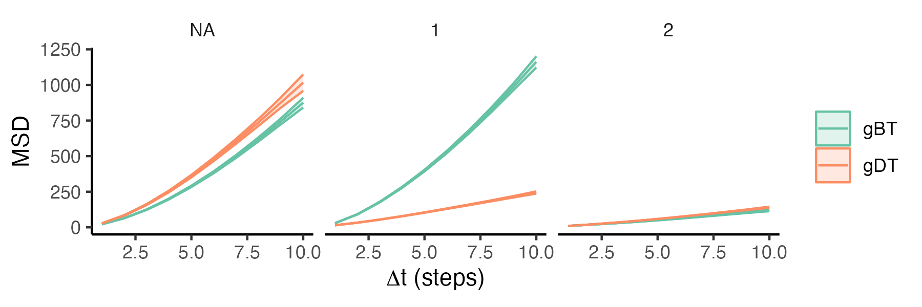
 1# compare msd on plot
 2tracks.DT.msd <- tracks.combine.dt(lapply(
 3  tracks.list, function(x) tracks.aggregate.fun(
 4    x, celltrackR::squareDisplacement,
 5    summary.FUN = "mean.se", add.time.delta = TRUE,
 6    subtracks.i = 10
 7    )
 8))
 9
10# focus specific images
11plot.uIDs <- c("LfVNe6", "2nFwDR", "fizPPH")
12
13# plot
14ggplot(tracks.DT.msd[uID %in% plot.uIDs] %>% left_join(exp.info),
15       aes(x = i, y = mean, color = cell_type, fill = cell_type)) +
16  geom_ribbon(aes(ymin = lower, ymax = upper),
17              alpha = 0.2) +
18  geom_line() +
19  labs(
20    x = expression(paste(Delta, "t (steps)")),
21    y = "MSD"
22  ) +
23  theme_classic() +
24  facet_wrap(~dpi) +
25  scale_color_brewer(palette = "Set2") +
26  scale_fill_brewer(palette = "Set2") +
27  theme(
28    legend.title = element_blank(),
29    strip.background = element_blank()
30  )